pak::pak("Permian-Global-Research/rsi")An overview of the rsi R package for retrieving satellite imagery and calculating spectral indices
Introduction
rsi is a recent R package developed by Michael Mahoney and funded by Permian Global Research. It offers features that simplify the process of acquiring spatial data from STAC (SpatioTemporal Asset Catalog) and calculating spectral indices based on such data. A unique feature of this package is its source for the indices. Instead of providing a static list of available formulas, rsi obtains them from Awesome Spectral Indices: a curated repository of over 200 indices covering multiple application domains. The combination of satellite imagery access through STAC and a constantly expanding spectral indices repository significantly simplifies remote sensing processes and creates new opportunities, including the automation of calculating spectral indices over a wide span of time and area.
Set up
rsi is available in development version on GitHub, which can be installed with pak.
To acquire the newest Awesome Spectral Indices dataset, we can call spectral_indices(). Calling it without passing any arguments will result in using cached version of the tibble, which is updated automatically once a day. This tibble contains column with indices formulas, which are using standardized band names.
library(rsi)
asi = spectral_indices(download_indices = TRUE)
asi
# A tibble: 231 × 9
application_domain bands contributor date_of_addition formula long_name
<chr> <list> <chr> <chr> <chr> <chr>
1 vegetation <chr [2]> https://gith… 2021-11-17 (N - 0… Aerosol …
2 vegetation <chr [2]> https://gith… 2021-11-17 (N - 0… Aerosol …
3 water <chr [6]> https://gith… 2022-09-22 (B + G… Augmente…
4 vegetation <chr [2]> https://gith… 2021-09-20 (1 / G… Anthocya…
5 vegetation <chr [3]> https://gith… 2022-04-08 N * ((… Anthocya…
6 vegetation <chr [4]> https://gith… 2021-05-11 (N - (… Atmosphe…
7 vegetation <chr [4]> https://gith… 2021-05-14 sla * … Adjusted…
8 vegetation <chr [2]> https://gith… 2022-04-08 (N * (… Advanced…
9 water <chr [4]> https://gith… 2021-09-18 4.0 * … Automate…
10 water <chr [5]> https://gith… 2021-09-18 B + 2.… Automate…
# ℹ 221 more rows
# ℹ 3 more variables: platforms <list>, reference <chr>, short_name <chr>Acquiring STAC data
rsi provides get_stac_data() function, built around the rstac package. It allows to connect to specified STAC source, and access data, based on selected attributes, like geospatial area of interest, date of acquisition of imagery, collection name, etc. For users convenience, rsi comes with additional functions that facilitate get_stac_data() function, providing necessary parameters, and limiting users input to specifying area of interest and a time frame of imagery. Those functions allow to access Landsat, Sentinel 1-2 imagery and digital elevation models (DEMs), available on Microsoft’s Planetary Computer.
Let’s start with creating our area of interest. get_stac_data() accepts sf objects from which it extracts boundaries, so we can load in already existing data source, or create our own. For this example, we will create area of interest of 5000 meters around a point in San Antonio.
library(sf)
san_antonio = st_point(c(-98.491142, 29.424349))
san_antonio = st_sfc(san_antonio, crs = "EPSG:4326")
san_antonio = st_buffer(st_transform(san_antonio, "EPSG:3081"), 5000)
Having specified the area of interest, we can create our query. We will start with downloading Landsat data for September and October 2023 and save it to a temporary file.
sa_landsat = get_landsat_imagery(
    san_antonio,
    start_date = "2023-09-01",
    end_date = "2023-10-31",
    output_filename = tempfile(fileext = ".tif")
)
sa_landsat
[1] "/tmp/Rtmppind2Y/file501082fbc26c0.tif"get_stac_data() and its child functions return the path to downloaded image. As a default, they create the composite image out of median values of all avaiable images for specified time span. We can specify other composite functions, like mean, sum, min or max. We can also not use composite function at all (composite_function = NULL), and obtain all available images for specified time span. Another default argument, passed in for mask_band, automatically masks clouds with NAs.
sa_sentinel2 = get_sentinel2_imagery(
    san_antonio,
    start_date = "2023-09-01",
    end_date = "2023-10-31",
    output_filename = tempfile(fileext = ".tif")
)
In this example, we download Sentinel 2 images for September and October 2023, mask out clouds, and create a composite image.
Let’s also obtain the DEM of our area.
sa_dem = get_dem(
    san_antonio,
    output_filename = tempfile(fileext = ".tif")
)
After downloading the images, we can load them into SpatRaster objects using rast(). rsi automatically assigns proper band names to it, which follow Awesome Spectral Indices standard.
library(terra)
sa_landsat_rast = terra::rast(sa_landsat)
sa_sentinel2_rast = terra::rast(sa_sentinel2)
sa_dem_rast = terra::rast(sa_dem)
sa_landsat_rast
class : SpatRaster
dimensions : 333, 333, 8 (nrow, ncol, nlyr)
resolution : 30, 30 (x, y)
extent : 1141170, 1151160, 803238.9, 813228.9 (xmin, xmax, ymin, ymax)
coord. ref. : NAD83 / Texas State Mapping System (EPSG:3081)
source : file501082fbc26c0.tif
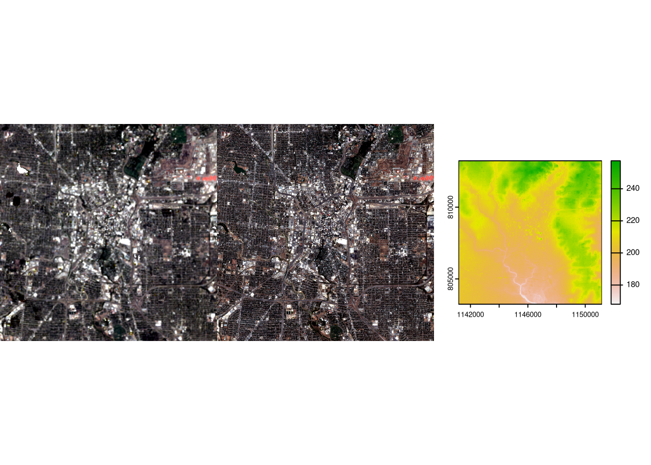
names : A, B, G, R, N, S1, ... We can plot the rasters together to compare Landsat and Sentinel images and visualize DEM.
par(mfrow = c(1, 3))
terra::plotRGB(sa_landsat_rast, r = 4, g = 3, b = 2, stretch = "lin")
terra::plotRGB(sa_sentinel2_rast, r = 4, g = 3, b = 2, stretch = "lin")
terra::plot(sa_dem_rast)
Calculating spectral indices
Having downloaded images, we can use them to calculate spectral indices. In this example, we will observe the change in vegetation between two dates for the Swarzędz area in Poland. Let’s start by creating a new area of interest.
swarzedz = st_point(c(17.108174, 52.405725))
swarzedz = st_set_crs(st_sfc(swarzedz), "EPSG:4326")
swarzedz = st_buffer(st_transform(swarzedz, "EPSG:2180"), 5000)
For the most accurate results, we will use Sentinel 2 data. The date span is set from July to September 2023. We will also pass in composite_function = NULL, so that all available images will be downloaded separately.
swarzedz_sentinel2_sep = get_sentinel2_imagery(
    swarzedz,
    start_date = "2023-07-01",
    end_date = "2023-09-30",
    output_filename = tempfile(fileext = ".tif"),
    composite_function = NULL
)

swarzedz_sentinel2_sep
[1] "/tmp/Rtmppind2Y/file5010818963908_2023-09-27T10:00:31.024000Z.tif"
[2] "/tmp/Rtmppind2Y/file5010818963908_2023-09-22T09:56:49.024000Z.tif"
[3] "/tmp/Rtmppind2Y/file5010818963908_2023-09-17T10:00:31.024000Z.tif"
[4] "/tmp/Rtmppind2Y/file5010818963908_2023-09-12T09:56:09.024000Z.tif"
[5] "/tmp/Rtmppind2Y/file5010818963908_2023-09-07T10:00:31.024000Z.tif"
[6] "/tmp/Rtmppind2Y/file5010818963908_2023-09-02T09:55:59.024000Z.tif"
[7] "/tmp/Rtmppind2Y/file5010818963908_2023-08-28T10:00:31.025000Z.tif"
[8] "/tmp/Rtmppind2Y/file5010818963908_2023-08-23T09:55:59.024000Z.tif"
[9] "/tmp/Rtmppind2Y/file5010818963908_2023-08-18T10:00:31.024000Z.tif"
[10] "/tmp/Rtmppind2Y/file5010818963908_2023-08-13T09:55:59.024000Z.tif"
[11] "/tmp/Rtmppind2Y/file5010818963908_2023-08-08T10:00:31.024000Z.tif"
[12] "/tmp/Rtmppind2Y/file5010818963908_2023-08-03T09:55:59.024000Z.tif"
[13] "/tmp/Rtmppind2Y/file5010818963908_2023-07-29T10:00:31.024000Z.tif"
[14] "/tmp/Rtmppind2Y/file5010818963908_2023-07-19T10:00:31.024000Z.tif"
[15] "/tmp/Rtmppind2Y/file5010818963908_2023-07-14T09:55:59.024000Z.tif"
[16] "/tmp/Rtmppind2Y/file5010818963908_2023-07-09T10:00:31.024000Z.tif"
[17] "/tmp/Rtmppind2Y/file5010818963908_2023-07-04T09:55:59.024000Z.tif"rsi allows for creating custom query functions using CQL2, which we can use to filter out products that do not meet our criteria. A common use case is filtering items based on their cloud coverage. For instance, if we want to download Sentinel-2 imagery with cloud cover below 25%, we can define our query function as follows:
sentinel2_25cc_qf <- function(bbox, stac_source, start_date, end_date, limit, ...) {
    geom <- rstac::cql2_bbox_as_geojson(bbox)
    datetime <- rstac::cql2_interval(start_date, end_date)
    request <- rstac::ext_filter(
        rstac::stac(stac_source),
        collection == "sentinel-2-l2a" &&
        t_intersects(datetime, {{datetime}}) &&
        s_intersects(geom, {{geom}}) &&
        platform == "Sentinel-2B" &&
        `eo:cloud_cover` < 25
        )
    rstac::items_fetch(rstac::post_request(request))
}
We could pass it in using the code get_stac_data(query_function = sentinel2_25cc_qf). This is an optional argument, as rsi provides a default query function. We can then continue our work with the results stored in swarzedz_sentinel2_sep, selecting two images that have low cloud coverage.
swarzedz_sentinel2_07_09 = terra::rast(swarzedz_sentinel2_sep[16])
swarzedz_sentinel2_09_27 = terra::rast(swarzedz_sentinel2_sep[1])rsi’s calculate_indices() requires a data frame of indices to calculate. Since we want to calculate NDVI, all we need to do is extract the row with NDVI’s formula. We can use the short_name column for that.
ndvi = asi[asi$short_name == "NDVI", ]
swarzedz_sentinel2_07_09_ndvi = calculate_indices(
    swarzedz_sentinel2_07_09,
    ndvi,
    output_filename = tempfile(fileext = ".tif")
)
swarzedz_sentinel2_09_27_ndvi = calculate_indices(
    swarzedz_sentinel2_09_27,
    ndvi,
    output_filename = tempfile(fileext = ".tif")
)
swarzedz_sentinel2_07_09_ndvi
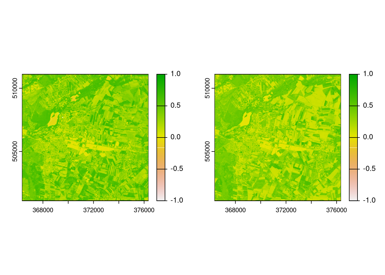
[1] "/tmp/Rtmppind2Y/file501084d439b94.tif"We now can plot both rasters to see the values that were calculated for both dates.
par(mfrow = c(1, 2))
swarzedz_sentinel2_07_09_ndvi_rast = terra::rast(swarzedz_sentinel2_07_09_ndvi)
swarzedz_sentinel2_09_27_ndvi_rast = terra::rast(swarzedz_sentinel2_09_27_ndvi)
terra::plot(swarzedz_sentinel2_07_09_ndvi_rast, range = c(-1, 1))
terra::plot(swarzedz_sentinel2_09_27_ndvi_rast, range = c(-1, 1))
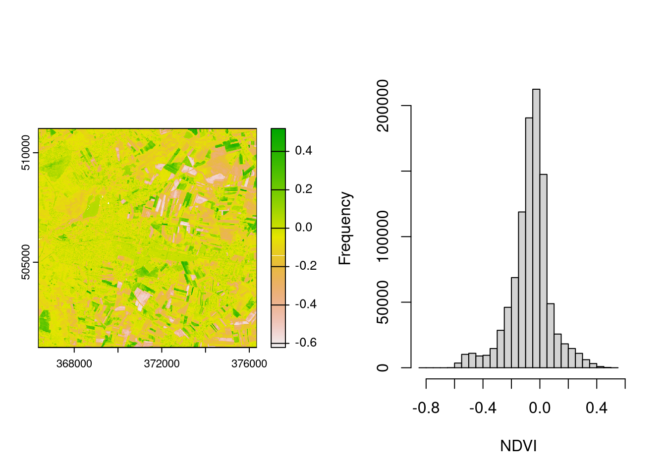
To better visualize the change in NDVI over time, we can create a difference raster. Values above 0 indicate that NDVI was higher on October 27 than on July 9. Values below 0 indicate that the NDVI values decreased on October 27, compared to July 9. Values equal to 0 mean that NDVI values haven’t changed over time.
par(mfrow = c(1, 2))
dif = swarzedz_sentinel2_09_27_ndvi_rast - swarzedz_sentinel2_07_09_ndvi_rast
terra::plot(dif)
hist(dif, main = "", xlab = "NDVI")
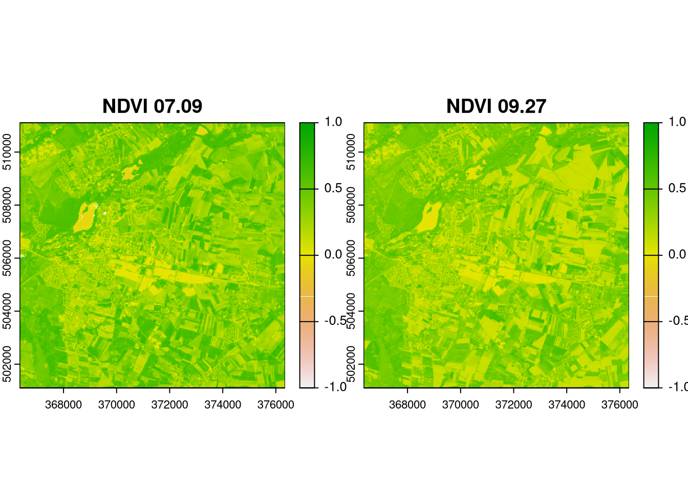
We can save both rasters as one, using stack_rasters() function.
stack = stack_rasters(
  c(
    swarzedz_sentinel2_07_09_ndvi,
    swarzedz_sentinel2_09_27_ndvi
  ),
  tempfile(fileext = ".vrt")
)
stack_rast = terra::rast(stack)
names(stack_rast) = c("NDVI 07.09", "NDVI 09.27")
stack_rast
class : SpatRaster
dimensions : 1000, 1000, 2 (nrow, ncol, nlyr)
resolution : 10, 10 (x, y)
extent : 366347.1, 376347.1, 501106.3, 511106.3 (xmin, xmax, ymin, ymax)
coord. ref. : ETRF2000-PL / CS92 (EPSG:2180)
source : file5010876ee0652.vrt
names : NDVI 07.09, NDVI 09.27
min values : -0.1237687, -0.5265973
max values : 0.7251614, 0.7040647 terra::plot(stack_rast, range = c(-1, 1))
Conclusion
The goal of this article was to demonstrate the capabilities of rsi package on the most common examples in remote sensing tasks. It’s current state already shows huge potential in many remote sensing applications. rsi provides functions which simplify processes of downloading satellite imagery and calculating spectral indices. If you want to learn more about rsi package, you can visit GitHub repository of the project.
While working on this article, I found many posibble features that could be added into rsi. An useful feature would be adding methods of simpler product filtering, based on cloud coverage and other parameters. Other feature could be focused on time series analysis, by calculating indices for each available item in selected time span.
I’m looking forward into the future developements of rsi.
Reuse
Citation
@online{rydzik2024,
  author = {Rydzik, Mateusz},
  title = {An Overview of the Rsi {R} Package for Retrieving Satellite
    Imagery and Calculating Spectral Indices},
  date = {2024-01-10},
  url = {https://geocompx.org/post/2024/rsi-bp1/},
  langid = {en}
}